For a specific task I had to solve I recently came across some interesting paper:
“Table detection is a crucial step in many document analysis applications as tables are used for presenting essential information to the reader in a structured manner. It is a hard problem due to varying layouts and encodings of the tables. Researchers have proposed numerous techniques for table detection based on layout analysis of documents. Most of these techniques fail to generalize because they rely on hand engineered features which are not robust to layout variations. In this paper, we have presented a deep learning based method for table detection. In the proposed method, document images are first pre-processed. These images are then fed to a Region Proposal Network followed by a fully connected neural network for table detection. The proposed method works with high precision on document images with varying layouts that include documents, research papers, and magazines. We have done our evaluations on publicly available UNLV dataset where it beats Tesseract’s state of the art table detection system by a significant margin.”
I decided to give it a try.
So — what do we need to implement this?
Required Libraries
Before we go on make sure you have everything installed to do be able to follow the steps described here.
The following will be required to follow the instructions:
- Python 3 (i use Anaconda)
- pandas
- Pillow
- opencv-python
- Luminoth (which will also install Tensorflow)
The Dataset
First, we need the data. Going through the paper I found some links that point to a website with XML files containing the ground truth for the UNLV dataset — but to keep things simple I will provide some already prepared dataset based on that 2 sources to start with.
You can download the dataset here — please extract in to a directory “data”.
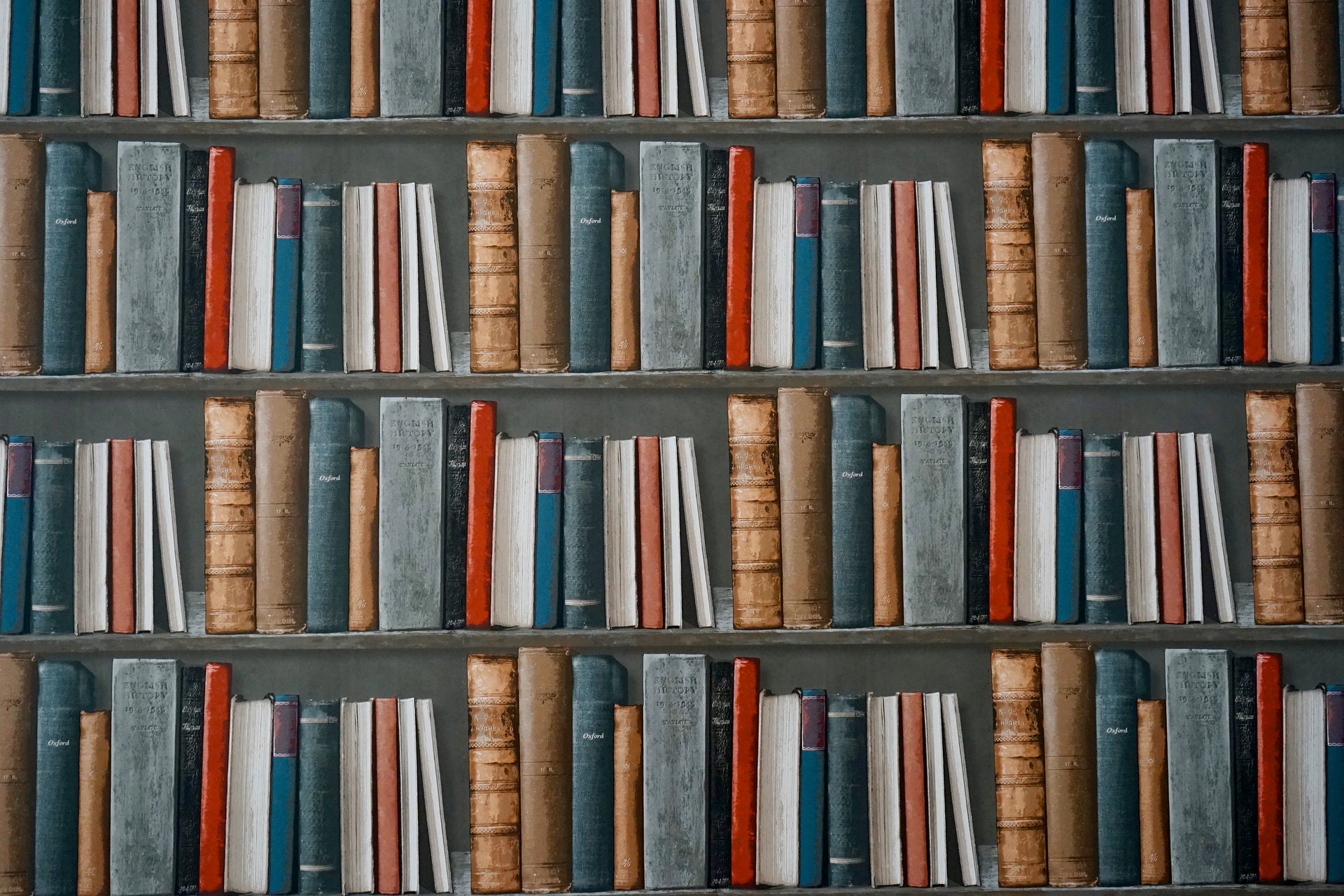
In the “data/images/” folder we have 403 image files from different types of documents like this one:

In addition to the images there are also 2 csv files with the ground truth data for this dataset. Each file has lines for each table found in each file, in the following format:
<filename>, <xmin>, <ymin>, <xmax>, <ymax>, <class> (in our case “class” will always be “table”)
The first lines of the train.csv file look like this:
0101_003.png,770,946,2070,2973,table
0110_099.png,270,1653,2280,2580,table
0113_013.png,303,343,2273,2953,table
0140_007.png,664,1782,1814,2076,table
0146_281.png,704,432,1744,1552,table
Preprocessing of images
The first part of the process is the preprocessing of the images. As the text elements in documents are very small and the used network is normally used for detecting real world objects in images we need to process the images to make the contents better understandable for the object detection network.
We will do this with in the following steps:
- open csv file
- read in all image file names in that file
for each image:
- preprocess image
- save image to data/train (for files from train.csv) or to data/val (for files from val.csv)
Let’s do this!
| import os | |
| import cv2 | |
| import pandas as pd | |
| root_dir = os.getcwd() | |
| file_list = ['train.csv', 'val.csv'] | |
| image_source_dir = os.path.join(root_dir, 'data/images/') | |
| data_root = os.path.join(root_dir, 'data') | |
| for file in file_list: | |
| image_target_dir = os.path.join(data_root, file.split(".")[0]) | |
| # read list of image files to process from file | |
| image_list = pd.read_csv(os.path.join(data_root, file), header=None)[0] | |
| print("Start preprocessing images") | |
| for image in image_list: | |
| # open image file | |
| img = cv2.imread(os.path.join(image_source_dir, image)) | |
| img = cv2.cvtColor(img, cv2.COLOR_BGR2GRAY) | |
| # perform transformations on image | |
| b = cv2.distanceTransform(img, distanceType=cv2.DIST_L2, maskSize=5) | |
| g = cv2.distanceTransform(img, distanceType=cv2.DIST_L1, maskSize=5) | |
| r = cv2.distanceTransform(img, distanceType=cv2.DIST_C, maskSize=5) | |
| # merge the transformed channels back to an image | |
| transformed_image = cv2.merge((b, g, r)) | |
| target_file = os.path.join(image_target_dir, image) | |
| print("Writing target file {}".format(target_file)) | |
| cv2.imwrite(target_file, transformed_image) |
After you have done this there should be 2 additional directories in you “data” folder — ”train” and “val”. These hold the preprocessed image files we later use for training and validating the results.
The images that folders now should look like this:

But before we start training the network there is one additional step that has to be done.
Creating TFRecords for training the network
Now that we have the preprocessed files the next step is to create the files needed as input for the training. Here we will use Luminoth framework for the first time.
As Luminoth is based on Tensorflow we need to create TFRecords which will be used as input for the training process. Luckily, Luminoth has some converters which you can use to transform your dataset accordingly.
To do this we will use the command line tool “lumi” which comes with Luminoth. In the directory where you placed the “data” folder open a terminal or command line and type:
| lumi dataset transform --type csv --data-dir data/ --output-dir tfdata/ --split train --split val --only-classes=table |
This will create a folder called “tfdata” with the TFRecords needed for the training of the network.
Training the network
To start the training of the network with luminoth we need to configure the training process.
This is done by writing a configuration file — there is a sample file available in the Luminoth Git repo, which I used to create a simple configuration (config.yml) for our task at hand:
| train: | |
| # Name used to identify the run. Data inside `job_dir` will be stored under | |
| # `run_name`. | |
| run_name: table-area-detection-0.1 | |
| # Base directory in which model checkpoints & summaries (for Tensorboard) will | |
| # be saved. | |
| job_dir: jobs/ | |
| save_checkpoint_secs: 10 | |
| save_summaries_secs: 10 | |
| # Number of epochs (complete dataset batches) to run. | |
| num_epochs: 10 | |
| dataset: | |
| type: object_detection | |
| # From which directory to read the dataset. | |
| dir: tfdata/classes-table/ | |
| image_preprocessing: | |
| min_size: 600 | |
| max_size: 1024 | |
| data_augmentation: | |
| - flip: | |
| left_right: True | |
| up_down: True | |
| prob: 0.5 | |
| model: | |
| type: fasterrcnn | |
| network: | |
| # Total number of classes to predict. | |
| num_classes: 1 |
Save this file to your working directory and we can start the training. Again we will use the tool “lumi” from Limunoth for this — so go to the terminal or command line (you should be in the folder with the data):
| lumi train -c config.yml |
This will start the training process and you should see output like this:

It can take quite a while to train the network — if the loss is getting close to 1.0 you can stop the training with <ctrl + c>.
Ok, now we have a trained network — what next?
Using the trained network to make predictions
To use the trained network to make prediction we first need to create a checkpoint.
In the terminal or commandline window type the following:
| lumi checkpoint create config.yml |
You see something similiar to this:
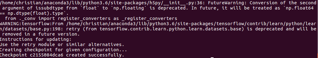
The last line with “Checkpoint c2155084dca6 created successfully.” holds the important information: the id of the created checkpoint (in this case c2155084dca6).
This is the identifier you need for the prediction for new images and if you want to load the model to the lumi webserver.
First we will use the command line tool to make a prediction (make sure to use the id of your checkpoint instead of c2155084dca6):
| lumi predict --checkpoint c2155084dca6 data/val/9541_023.png |
You should see something like the following:

The interesting part for us is “bbox” — the numbers show the coordinates of the table area whith x0 = 160, y0 = 657 (upper left corner of the area) and x1 = 2346, x2 = 2211 (lower right corner of the area). This information can be used to mark the area in the original, unprocessed image and looks like this:

So the network seems to have a good idea where the table can be found on that page.
You can try that on your own — take the predict command above together with the id of your trained checkpoint and use an image tool of your choice to draw an area with the given coordinates on the image. You will see that it will fit the area nicely around the table on the pages.
If you want a quick view on the prediction you can also use the small web application that comes with Luminoth, but this can only be used with the preprocessed files.
To use it start the web server with the command (again — make sure to use the id of your checkpoint instead of c2155084dca6):
| lumi server web --checkpoint c2155084dca6 |
This will start the webserver that comes with Luminoth where you can upload the preprocessed images to see the predictions which looks like this:
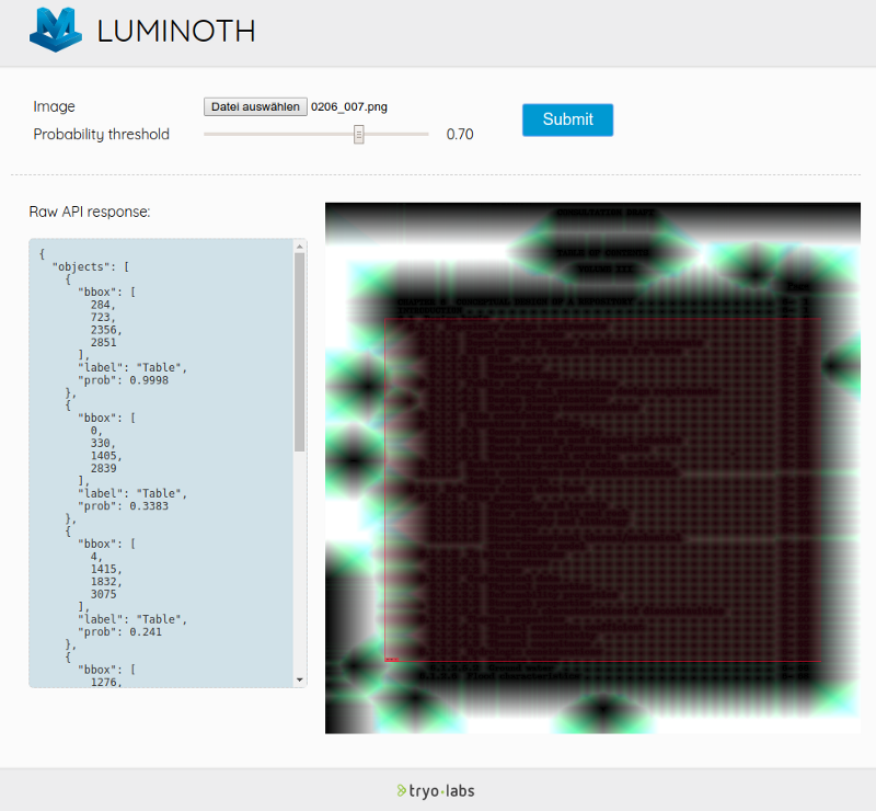
Although this has to be done using the preprocessed images you still get an idea of how good or bad the network detects the table areas.
Conclusion
In this article I gave a brief overview on how to implement the concept described in the research paper.
But detecting the table area alone is not of practical use — you still need some tools or libraries that can use this area definitions as input to actually get the content of the tables.
For those of you who want to go further on this I can recommend to take a look at tabula-py, a Python library that can take the area definitions as input to improve accuracy of extracting the data of the tables.
Hmm…. maybe a good topic for a second article? 😉
